GPU Ray Tracing

In this blog post, I will demonstrate how to use a GPU in order to accelerate the ray tracing code developed in previous blog posts. Specifically in this blog post I will be using Numba’s CUDA extension to write a CUDA kernel for the ray tracing code. Numba has support for parallel programming using both AMD and Nvidia GPUs, although this post will focus on development for a Nvidia GPU.

Why expand beyond CPUs?

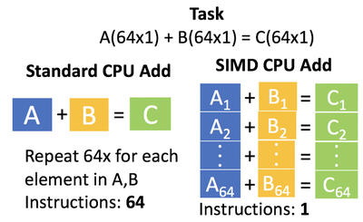
CPUs today are made to do many different tasks at once. This is baked into the heart of many operating systems today where a scheduler determines how to allocate the CPUs time to best use it. Currently, the amount of tasks that can be done at once is limited by the number of cores on the CPU. There is a slight caveat to this, today’s CPUs have Single Instruction Multiple Data(SIMD) instructions. SIMD instructions allow for a single instruction to operate on multiple pieces of data at once. For example, one could perform a parallel add of a vector A+B (Fig. 1). Each of these SIMD instructions has a max # elements it can handle at once, the latest SIMD instruction is AVX-512. SIMD instruction provides speed up but still, there is a need to perform more computation per clock cycle.

GPUs

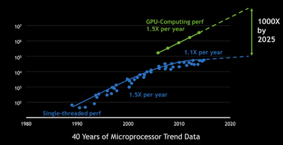
One great alternative to CPUs for computing is GPUs. GPUs over the past years have become a major player in computing power(Fig. 2). On GPUs, you have control over what code, called a kernel on a GPU, is running and don’t have to worry about performing many different tasks. The reason why is a GPU has many independent computing units(ALUs) that can perform computations. Specifically, each GPU has a different amount of these processors, for example on the GTX 1070 used in this investigation 1920 computing cores are available. A GPU works off a single instruction multiple threads model where a single instruction gets executed by multiple different computing units. An example of this is an add instruction could be performed by multiple different threads on a GPU. The big difference between a GPU and CPU is a GPU performs many of the same computations over many different cores, as opposed to a CPU which is built to do many different tasks.

Programming Model for a GPU

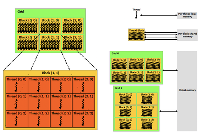
The programming model for a GPU consists of writing a modular function that can be applied to many pieces of data. A GPU consists of many different tiers of memory which a given thread(single executing block of code) can access, for example, a thread can access A) Global Data, B) Block of Thread Data, C) Thread Local Data. This leads to another concept of a GPU which is the layout of different threads onto a GPU. A GPU runs many different threads which are grouped into blocks which are further grouped into grids(Fig. 3). The way that a GPU schedules these grids is by the concept of warps. A warp is a group of X number of threads that are scheduled onto a streaming processor.

X-ray GPU Computing

One way to apply the GPU programming model to the X-ray forward solver is to parallelize each thread to perform computation for a single ray. For this, the main loop function instead of performing a loop over all the pixels should be changed to use the CUDA thread index. CUDA will run this program with a varying number of threads in a specified number of dimensions.
Old way of indexing rays:

for z in range(0, Mx * My):
  j = z % Mx  # y direction pixel
  i = int(z / Mx)  # x direction pixel

New way of indexing rays:

i, j = cuda.grid(2) # Create thread indices i, j

For example in the above, cuda.grid(2) will create index i, j which will be used to index each ray starting from the detector pixel. Then in CUDA one must launch each function with main_loop[(25, 25), (25, 25), stream](h_image_params, d_mu, d_detector). The specialized part of this function call is the four numbers given, which specify the number of blocks per thread and number of blocks to launch. One important note, if the threads are greater than the number of indexed dimensions an if statement is needed to return on unused threads. Additionally, another change to the overall code is rather than using vectorized NumPy function, one has to write in looped functions that use the Math library. This is due to the fact that NumPy creates new memory and this violates the GPU programming model. Additionally, the one move in cube function has to be ported to the GPU programming model. For this, again the function was ported to not use NumPy and it was created as a device function. For device functions, one has to call this function from another function already running on a CUDA device.

Tweaks

While porting the algorithm over to the GPU, I ran into multiple issues with the algorithm. First, the algorithm would never end meaning the rays weren’t reaching the detector. Then, different results were being obtained than the Numba CPU results. Multiple different tweaks needed to be performed to get the algorithm to function. Additionally, Numba has a CUDA simulator and the algorithm worked fine on this without tweaks but failed when moving to the GPU. One of the first problems with the algorithm was rays not moving forward when one of the positions was close to zero. A fix for this was an if statement checked if the position was close to zero and added a small amount to that number in order to keep the ray marching.

if -.0001 < pos[0] < .0001:
    pos[0] += .0001

Another problem was results from functions would not be copied into variables. The fix for this was to create a new temporary for function results then copy these results into the variable I wanted to copy into.

for k in range(3): 
    pos[k] = p1[k]

One final problem was in the one move in cube function, CUDA needed a small decrement from the assigned value for the function to continue marching.

htime[i] = abs((math.floor(p0[i]) - p0[i] - 1e-4) / v[i])

All of these tweaks were different things that I found while trying to debug the program. In the end, I compared the Numba and CUDA results on a 300x300 detector and only 4 pixels differed in values. If you have any idea how to fix some of these, please email me!

Timing

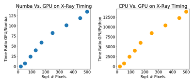
After getting this code in a runnable form, I compared the CUDA Numba, Numba and Python version in terms of running time. Looking at the CUDA results one can see the CUDA speedup increases with the number of pixels. The reason for this is the amortization of various things on the GPU with a larger number of pixels. Looking at the speed up the CUDA code is by far the fastest with a speedup of 6700x compared to Python code and 67x compared to Numba.

Checkout the code for this here Thanks for following my X-ray tracing miniseries!