X-ray Imaging

This post will review the concepts behind medical imaging and the forward model used in X-ray imaging. Additionally, this tutorial will explain the development of the forward model in Python.

Background

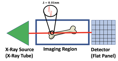
X-rays are one type of electromagnetic radiation used in medical imaging. The setup of an X-ray imaging systems consists of an X-ray transmitter (X-ray Tube) and a detector (Flat Panel Detector). X-rays interact with any matter between the transmitter and detector, for medical imaging this could be a femur, stomach or another area on the patient. As a result of an object in the imaging region, the transmitted X-rays lose energy due to photon interactions with matter and produce a projected pattern of this matter on the detector. One way to describe the amount of energy that is lost per unit length by the transmitted X-ray is $\mu$ which is the linear attenuation coefficient. The linear attenuation coefficient is different in every part of the body due to the different matter in each of these regions.

X-ray Imaging Model

One way to describe X-ray imaging is it produces a projection image of the combined linear attenuation coefficient onto the detector. This can be seen by the X-ray modeling equation of $$ I_0e^{-\mu(i,j,k)L(i,j,k)} \tag{Eq. 1}\label{eq:one} $$
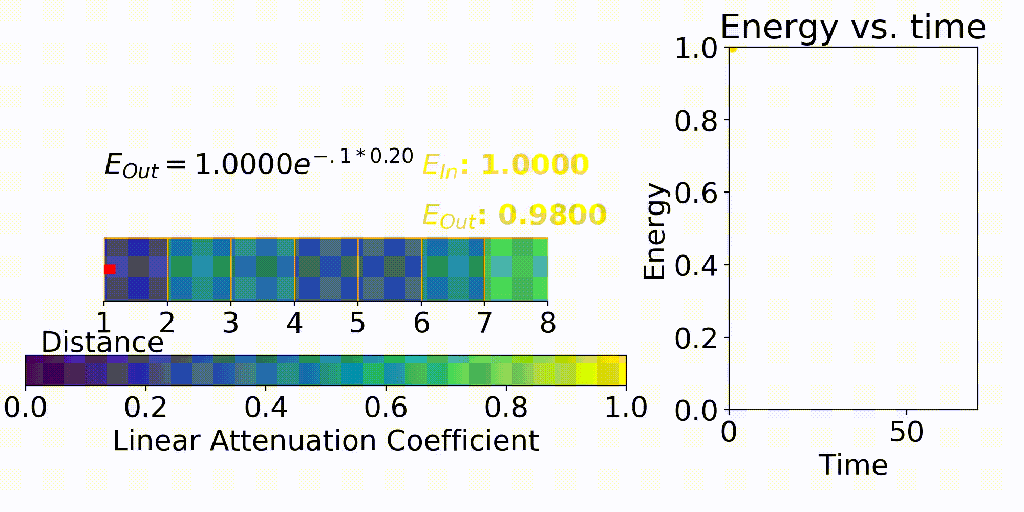
This first term in the equation is $I_0$ which is the energy emitted from the X-ray source. The next term $\mu$ is the previously stated linear attenuation coefficient in a certain X, Y, Z coordinate and L is the path length. Eq. 1 is the forward model which describes the energy received at a detector pixel given an initial X-ray energy and discretized model for the linear attenuation coefficients. This forward model is important for testing out different X-ray system parameters such as beam energy, beam filtering, and many others.

Discretization

Discretization is a process used to take a continuous space and break it down into a manageable subspace that can fit into the memory on a computer. The reason why this is necessary for our forward model is to make the problem computationally tractable and sampling for linear attenuation coefficient matrices are discrete.
One example of discretization can be seen in the Fig. 3, where we break up the imaging space into discrete cubes (seen in purple). Each of these chunks is an area of the body in the 2D case that represents the linear attenuation coefficient in that area. One factor to consider when performing discretization is the resolution of each of these chunks. In the below figure, some chunks have both bone and air present which will result in a fuzzy representation of this area. When performing imaging it is important to have the right discretization to best resolve the various areas of the patient.

Ray Tracing

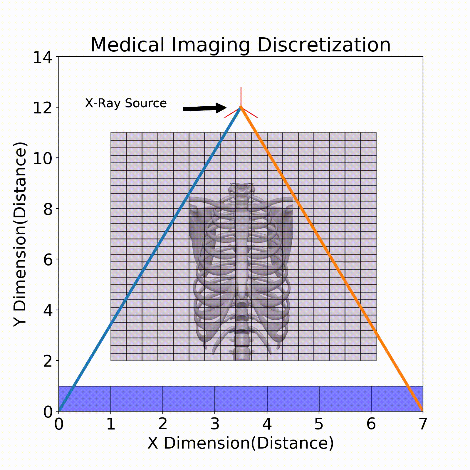
The model that relates the energy between an X-ray source and a detector pixel is a recursive implementation of Eq. 1. To apply this model, ray tracing is performed where a ray is stepped from source to detector pixel(Fig. 3). This ray will move along its direction vector and when it hits a new discretization in the imaging region will lose energy according to Eq. 1. A factor into the energy lost is the path length which is the distance the X-ray traveled within the discretization. This factor comes from the linear attenuation coefficient which is energy loss per unit length, so this path length is used to describe the amount of energy lost in that chunk.

Computational Model

The below shows an example of the 3D model that could be used for the above figure. Initially, we have the main loop function which will calculate the energy at each pixel location. To perform this calculation first, the direction vector between a pixel and the source is calculated. A ray is then initialized at the source and moves towards the next discretization cube on the direction vector. The move cube function is what performs the movement from one cube to another and returns the position and distance to the next cube. For each of these moves, the position is verified to be in the imaging region if, so it will perform the energy loss calculation, otherwise, it will continue the chunk movement (since outside of the imaging region is air where no energy is lost). To perform this energy calculation, Eq. 1 is used.

def main_loop(Nx, Ny, Nz, Mx, My, D, h, orginOffset, ep, mu):
    '''
    Ray tracing from end point to all pixels, calculates energy at every pixels
    Args:
        Nx: uint imaging volume length in x direction
        Ny: uint imaging volume length in y direction
        Nz: uint imaging volume length in z direction
        Mx: uint number of pixels in x direction
        My: uint number of pixels in y direction
        D: uint pixel length
        h: uint distance from detector to bottom of imaging volume
        orginOffset: np.array 1x2 offset origin for detector position start (X,Y)
        ep: np.array 1x3 location of the X-ray source (X,Y,Z)
        mu: np.array 1x3 normalized linear attenuation coefficient matrix (Nx,Ny,Nz)
    Returns:
        detector: np.array 1x3 next cube position (X,Y,Z)
    '''
    detector = np.zeros((Mx, My), dtype=np.float32) 
    for i in range(Mx): 
        for j in range(My):
            pos = np.array([orginOffset[0] + i * D, orginOffset[1] + D * j, 0], dtype=np.float32) # pixel location
            direction = ((ep - pos) / np.linalg.norm(ep - pos)).astype(np.float32) # normalized direction vector to source
            direction[direction == 0] = 1e-16 # need this for divide by 0 errors
            L = 1 # initial energy
            h_z = h + Nz
            while pos[2] < h_z:  # loop until the end of imaging volume
                pos, dist = onemove_in_cube(pos, dir)   # move to next cube
                if 0 <= pos[0] < Nx and 0 <= pos[1] < Ny and h <= pos[2] < h_z: # if in imaging volume calculate energy using mu
                    L *= np.exp(mu[int(np.floor(pos[0])),int(np.floor(pos[1])) , int(np.floor(pos[2] - h))] * dist)
            detector[i][j] = L # detector pixel location equals lasting energy
    return detector

Cube Marcher

The cube marching function will take the current position and find the next cube for which the ray will land. The first line in this function will calculate the distance to hit the different dimensions of the cube (X, Y, Z). Then, we want to use the minimum times as this is where the ray intersects first. After that, we want to record the distance to get to that new location and update the new position. Note this new position has an added epsilon for the next update because some next iterations result in endless looping.

def onemove_in_cube(p0, v):
    '''
    This is a function that moves from a given position p0 in direction v to another cube in a 1x1x1mm setup
    Args:
        p0: np.array 1x3 start position (X,Y,Z)
        v: np.array 1x3 normalized(1) direction vector (X,Y,Z)
    Returns:
        times: np.array 1x3 next cube position (X,Y,Z)
        dist: uint distance to the next cube position
    '''
    times = np.abs((np.floor(p0) - p0 + (v > 0)) / v)  # find time vector to new position
    minLoc = np.argmin(times)  # find dimension with minimum time
    dist = times[minLoc]  # find min distance
    times = p0 + dist * v  # calculate new position
    times[minLoc] = round(times[minLoc]) + np.spacing(abs(times[minLoc])) * np.sign(v[minLoc]) # updated location needs an epsilon to stop an occurrence of endless loop 
    return times, dist

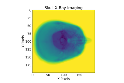
After performing all the above steps, one example of using these functions on a skull’s linear attenuation coefficients can be seen below:

For full code/constants definitions/imaging model diagram see Github, this code also has optimizations present which you can read about here.
That wraps up the basic model of X-ray imaging. One problem with the above Python implementation is it takes a long time to perform the forward model. In my next blog post, I will review Numba a library to accelerate your Python code and apply it to the X-ray imaging problem.